Style your R
Advanced R by Hadley Wickham is a great resource for people working with R. It provides a good overview and a much deeper dive into some components of functionality within the R programming language. This short article goes into some of the major concepts in the Style section and builds on them, along with my own suggestions.
File Naming
Hadley makes the excellent suggestion that file names should be clear and meaningful. I want to back up though, because I think proper directory structure is the place to start here. I make the same point over and over, when you start a project it’s important to think about how your project is going to look. A folder with ten R files is going to look messy. Where are your input data files going? Where are the output files going? Jenny Bryan has a great link on her website and there is an excellent review from Software Carpentry for Good Enough Practices.
Basically, I like to see a repository that looks like this:
.
|\- data
|    \- input   [directory]
|    \- output  [directory]
|\- R           [directory]
|\- figures     [directory]
|-- main-R-file.R (or Rmd)
|-- OTHER (github/etc) FILES
This then eliminates the need for Hadley’s second recommendation about file naming, that sequential files be numbered, e.g., 01_load-data.R, 02_run-analysis.R, 03_make-figures.R.
If you have a nice clean directory structure you can create a “control” file that does the following:
# Parent file, this file calls the other files in order:

source("R/load-data.R")
source("R/run-analysis.R")
source("R/make-figures.R")
The advantage here is in simplicity. If you were running each of those files in order you’d basically be doing the same thing anyway, so why not just formalize it. That way your directory structure and file names are also cleaner, and you can run the whole thing from the command line easily with one command:
R < main-R-file.R
Now R will run each of those source() calls, and you’ll have fewer files in each directory. There are other solutions, using RMarkdown, or make files. I use RMarkdown extensively, because I like adding text here and there, and I think you can do some cool stuff with RMarkdown, but Gavin Simpson got me interested in looking at make files a little further and I found this interesting make tutorial by Karl Broman, and a useful page called “Why Use Make” that explains why you should use make files.
Object Names
I don’t have many suggestions here, I think that the general ideas here are excellent (obviously). THe only thing I’d suggest adding here is to try to limit the number of global variables in your namespace.
In some cases the use of general variable names (like x, or i or counter) is unavoidable, and also advantageous. The problem comes when you have multiple R files used in your analysis, it becomes possible to start coding in such a way that you might expect x to behave one way in one place, but have made an upstream change where you use x in a new and unique way, that changes its behaviour later:
# I want to generate some random numbers:
x <- runif(1000)
y <- runif(1000)

plot(x, y)

# Some extra code
# . . .
# I now expect to use those random numbers to generate noise in a dataset

some_prediction <- predicted_values + x
But then a colleague adds a chunk of code to plot some spatial data in a new file called plot_zebra.R and sticks in a source() call in your code where the ellipsis were:
zebra_data <- read.csv("data/zebra-crossings.csv")
x <- zebra_data$long
y <- zebra_data$lat
counts <- zebra_data$counts
png("figures/zebra-crossings.png")
plot(x, y, col = counts)
dev.off()
There are a lot of problems with this code, for example, as Gavin Simpson points out here:
@sjGoring (apart from terrible habit of pulling out objects for no reason: plot(lat ~ long, data = zebras, col = zebras$counts)...
— Gavin Simpson (@ucfagls) October 17, 2016
But you’re not always going to be working with experts, and there are cases where we might accept imperfect code, so long as it’s self-contained. Regardless, let’s accept our collaborators suggestion, and assume that they are contributing as best they can.
So what’s the problem? If this code is stuck into a seperate file and called using source() in the upper code block, I might never know why my values for some_prediction are suddenly so strange. This is one of the problems of dealing with complex projects, and I’ve run into it a number of times. Using common, or default variable names, and burying things into multiple files can often result in unexpected behaviour. You might think of looking at the assertthat package as one possible solution.
Another solution is to wrap externally sourced code into functions and then source() the code, only calling the function in the main body of the script. Pass in only the most important details, and pass out only the most critical outputs (or NULL). Every call within the function will only live in the local environment of the function, an is extinguished once the function runs:
plot_zebras <- function(){
  zebra_data <- read.csv("data/zebra-crossings.csv")
  x <- zebra_data$long
  y <- zebra_data$lat
  counts <- zebra_data$counts
  png("figures/zebra-crossings.png")
  plot(x, y, col = counts)
  dev.off()
}
There are issues with this specific function, as Barry Rowlingson pointed out:
@sjGoring @ucfagls @MozillaScience @UBC @minisciencegirl suppose you want to see that plot on screen? Or send to PDF?
— Barry Rowlingson (@geospacedman) October 17, 2016
The plot_zebras() function really doesn’t do anything except make the plot and write it to file. We could improve the function by explicitly returning objects, adding if/else controls and changing the input parameters. In this case, let’s assume that all that is required in this case is a plot of the zebra data.
In this case, the changes to x and y that occured in the Global environment in the last code block happen internally within the environment of the function. Now, your code in the main file would look like this:
# I want to generate some random numbers:
x <- runif(1000)
y <- runif(1000)

plot(x, y)

# Some extra code

source("plot_zebras.R")
plot_zebras()

# I now expect to use those random numbers to generate noise in a dataset

some_prediction <- predicted_values + x
Your code would run the way you expect, without unexpected changes to x and y. I might still question your insistence on using these variables this way, but at least you’re not having unexpected behaviour.
In our meeting gvdr pointed out that it really is simple to change the variable names to something like zebra_x and zebra_y, or something. This is true, and we could also easily change indices in for loops to taxon_loop_index or something. In many cases this may reduce confusion. I feel like changing from the very standard convention of using i, j, and k in loops is potentially problematic, and x has value as a generic input parameter for functions. So, this is probably more a judgement call than anything.
Styling Code
I have two suggestions, one is the lintr package and the other is recommended in the Style Chapter, the formatR package.
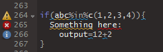
I really like lintr. It automatically integrates into your RStudio edit panel, so you can see mistakes right away:
There are other code profiling tools you could use, like codetools, but I think that’s a discussion, best suited for somewhere else.
Comments
Comments are good, comments are important, but too many comments are too much. That said, as with other elements of style, it all depends on your audience. If you are providing code to someone just starting out in R, then you may want to code extensively. This is an example of some code I sent to someone new to R looking to download all pollen data from Neotoma (we were getting a strange bug that seemed to have to do with an internet connection causing some of the downloads to fail, hence the use of try):
library(neotoma)

# Find all the pollen datasets in the world:
pollen_ds <- get_dataset(datasettype = "pollen")

# Now download them all. This will take forever.
pollen_dl <- get_download(pollen_ds)

# This compiles each record separately, if there's an error the `try` function will catch it.
compiled_dl <- lapply(pollen_dl, function(x)try(compile_download(x)))

# This gives you a vector of whether or not the results failed, so you can go back & check them, or send me the list :)
# everything should be a data.frame except the failures, which should be a "try-error"
which_failed <- sapply(compiled_dl, function(x)class(x)[1])

# This then removes any failures from the long list of data.frames:
for (i in length(compiled_dl):1) { if (which_failed[[i]] == 'try-error') compiled_dl[[i]] <- NULL }

# This needs the R package dplyr,
big_matrix <- dplyr::bind_rows(compiled_dl)

# And voila!
write.csv(big_matrix, "all_pollen_output.csv")
Lots of comments. But we were doing something unusual, they didn’t have much experience with either the neotoma R package or R itself, and I was hoping to provide some extra context.
When you start working on large projects this kind of intensive commenting becomes unwieldy though. It’s important to remember that good code should be self descriptive. Descriptive code involves careful naming of files, functions and variables and good flow control. For example, if we revisit our zebra code-block from above:
z_dat <- read.csv("data/z-cross.csv")
acrs <- z_dat$ln
updwn <- z_dat$lt
cnts <- z_dat$num
png("figures/z-cross.png")
plot(acrs, updwn, col = cnts)
dev.off()
We might require lots of comments to have it make sense to the next person who reads it. I mean, I guess I see what you’re doing, but it could get very complicated. Especially if all your project code looks like this!
So we could add comments:
# Read in Zebra crossing data:
z_dat <- read.csv("data/z-cross.csv")

# Get the latitudes & longitudes:
acrs <- z_dat$ln
updwn <- z_dat$lt

# These are the counts
cnts <- z_dat$num

# Now get it to plot:
png("figures/z-cross.png")
plot(acrs, updwn, col = cnts)
dev.off()
Which is better, but if we just had the function as it was, the meaning and utility would be clear:
plot_zebras <- function(){
  zebra_data <- read.csv("data/zebra-crossings.csv")
  x <- zebra_data$long
  y <- zebra_data$lat
  counts <- zebra_data$counts
  png("figures/zebra-crossings.png")
  plot(x, y, col = counts)
  dev.off()
}
The function name tells you the intent. The variable names are clear and the functions are straightforward.
In looking at the comments section I again depart a bit from Hadley. I don’t like the recommendation of using long “spacing” comment lines. I used to use them a lot, preferring long lines of ###### octothorpes to break up my code:
some <- code + other_code

# Plotting -----------------------------------------------

code_needed(to_plot,
			... )
and_some <- stuff(to(make(the)), plots)

plot(all_the, code, to_plot, goes, here)

# More Analysis ------------------------------------------

some <- more_code
and <- some_functions()
...
I actually think it makes code look a bit ugly. I’d rather see those sections be blocked into unique files to make navigation easier. So the code might look like this:
some <- code + other_code

source("plot_code.R")
plot_code()

some <- more_code
and <- some_functions()
...
That’s entirely personal though. In general my code is embedded within RMarkdown files, so many of these chunks of code are broken out using text blocks anyway, and there, my priority is often making the code chunks as short as possible, to maintain the flow of writing. This is another reason for my heavy dependence on source() calls.
Conclusion
The last point is that, as with all style, much about style in your R code is personal. There are certainly broad lessons that will help you improve your practice, but you need to find what works best for you.
One reason to adopt broader standards is that it makes collaboration much easier, especially as you progress in your coding activities. It is hard working on a project where there is no agreed upon style, and where each person spends as much time revising the other’s code as they do adding new code. If you’re finding that you have a hard time reading your own code, then maybe you need to take a step back and look at your coding style. Are there things you could be doing to improve? If you’re anything like me, then yes, there always is.